Chapter 6: Vector Visualization
Scenarios
Below are several scenarios that illustrate techniques for the visualization of 2D and 3D vector datasets described in Chapter 6. As always, make sure to study also the complementary techniques described in the source code samples for Chapter 6.
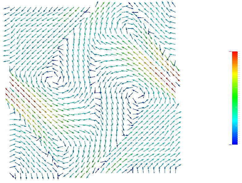
2D hedgehogs
This scenario visualizes a 2D vector field using arrow hedgehog glyphs, scaled and colored to reflect the orientation, respectively magnitude, of the vector field.
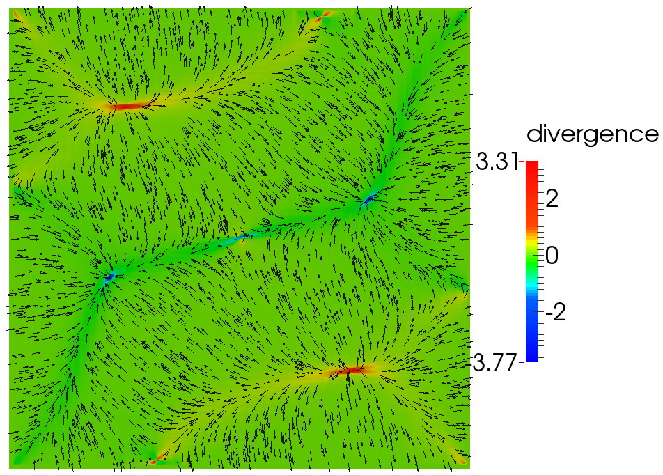
Divergence
This scenario visualizes a 2D vector field by plotting a color-mapped image of the divergence of the vector field. This emphasizes the sources and sinks of the field. Additionally, hedgehog glyphs are overlaid with the color-mapped divergence field.
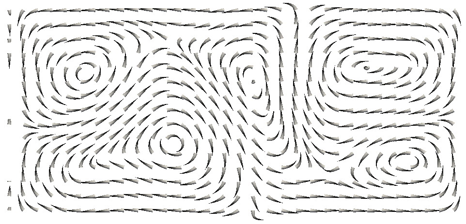
Curved glyphs
This scenario visualizes a 2D vector field by using curved arrow glyphs. The glyphs indicate the direction of the vector field by a combination of shape and thickness, constructed using short streamtubes whose thickness is scaled along the flow direction.
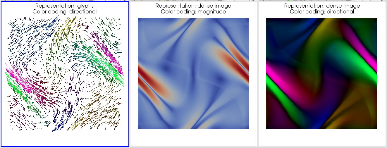
2D vector visualization variations
This scenario visualizes a 2D vector field using three combinations of techniques
- randomly-seeded arrow glyphs, color-coded by orientation, scaled by magnitude
- color-coded scalar visualization of the vector field magnitude
- hue coded scalar visualization of the vector field orientation
3D hedgehogs
This scenario visualizes a 3D vector field using line hedgehog glyphs, scaled and colored to reflect the orientation, respectively magnitude, of the vector field. Various colormaps and transparency maps are used, to illustrate the challenges and solutions related to tackling 3D occlusion.
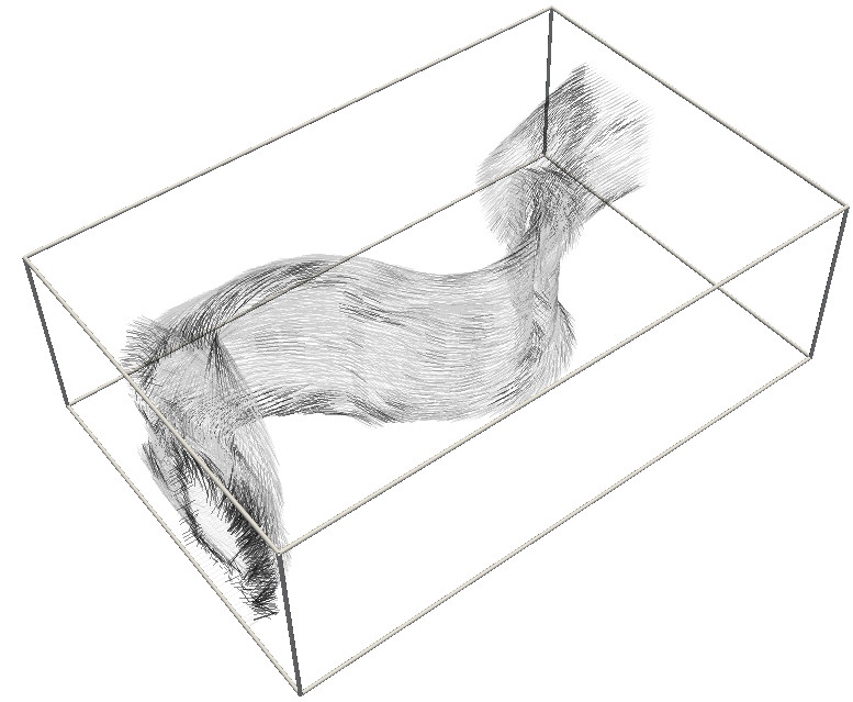
3D transparent hedgehogs
This scenario visualizes a 3D vector field using line hedgehog glyphs. An isosurface of the velocity magnitude is extracted first. Next, line hedgehogs are shown for the data points on this isosurface, using alpha blending to limit 3D occlusion effects.
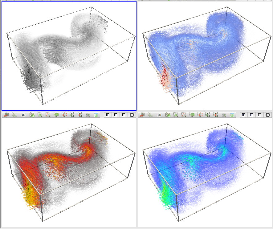
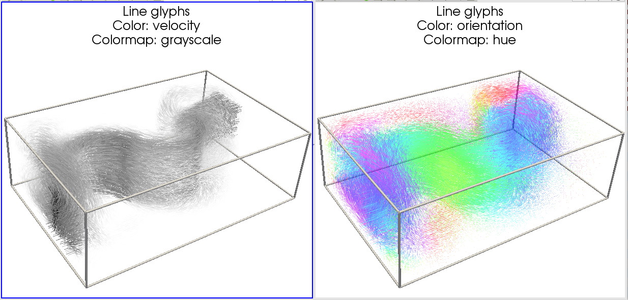
3D hedgehogs and color mapping
This scenario visualizes a 3D vector field using line hedgehog glyphs. Two color and alpha mapping variations are shown
- a grayscale map is used to show the vector magnitude
- a hue map is used to show the vector orientation
Velocity surfaces
This scenario visualizes a 3D vector field using a combination of techniques. First, a constant velocity-magnitude surface is extracted, corresponding to a high-speed flow region. Next, hedgehogs are plotted for points belonging to this surface, to show the flow direction. Finally, the surface is color-coded on the angle between the flow and the surface normal, indicating the direction of the flow with respect to the surface shape.

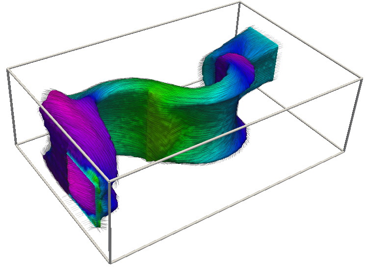
Velocity surfaces 2
This scenario is a variation on the previous one. First, a constant velocity-magnitude surface is extracted, corresponding to a high-speed flow region. Next, hedgehogs are plotted for points belonging to this surface, to show the flow direction. Finally, the surface is color-coded on the orientation of the flow on the surface, using a hue colormap.
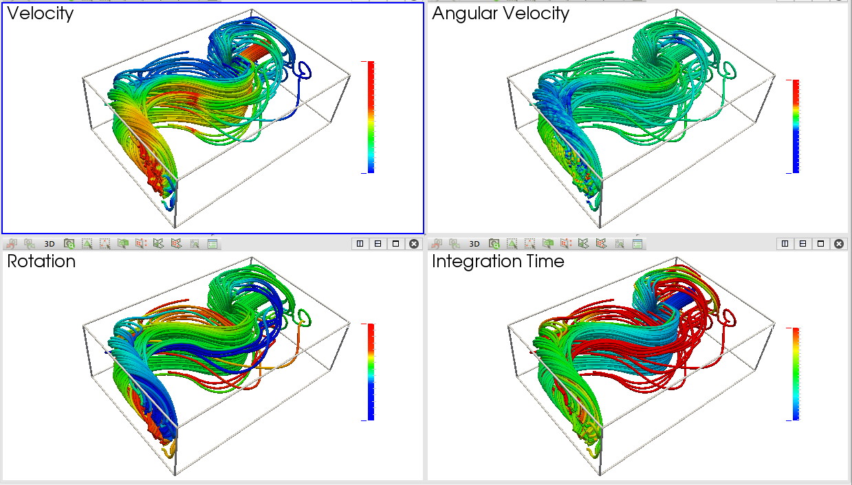
Color-coded stream tubes
This scenario demonstrates the use of stream tubes for the visualization of 3D vector fields. Given a flow field, the inflow region is densely seeded with streamlines. Next, constant-thickness stream tubes are constructed from these streamlines. Finally, four different scalar fields describing flow quantities (velocity, angular velocity, rotation, and integration time) are color mapped on the stream tubes.
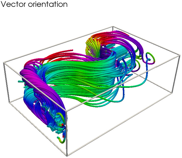
Color-coded stream tubes 2
This scenario is a variation on the previous one. Given a 3D flow field, the inflow region is densely seeded with streamlines. Next, constant-thickness stream tubes are constructed from these streamlines. Finally, the stream tubes are colored using a directional colormap to show the flow orientation.
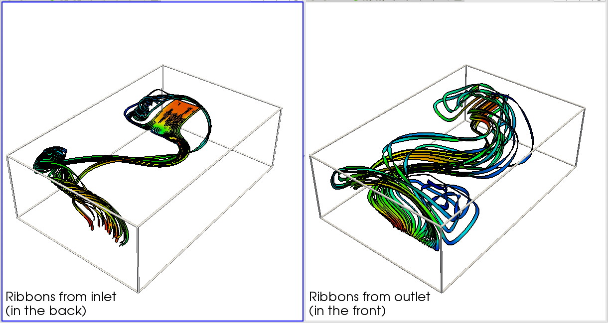
Stream ribbons
This scenario shows the usage of stream ribbons for visualizing a 3D flow field. The inflow and outflow regions are densely seeded with streamlines. Next, constant-thickness stream ribbons are constructed from these streamlines, resulting in two separate stream ribbon sets. Finally, the stream ribbons are colored to show the velocity magnitude.
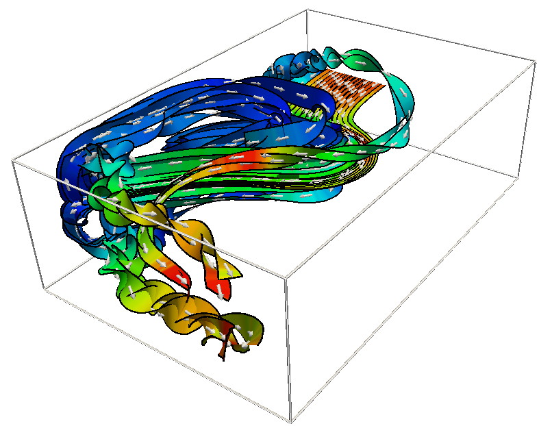
Stream ribbons 2
This scenario is a variation on the previous one. The inflow region of a 3D flow field is densely seeded with streamlines. Next, constant-thickness stream ribbons are constructed from these streamlines. The stream ribbons are colored to show the velocity magnitude. Finally, arrow glyphs are added to the streamlines, following a dashed pattern, to indicate the flow direction.
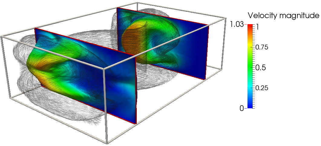
Warped planes
This scenario demonstrates the use of warped planes. For a 3D flow field, two planes are constructed roughly perpendicular to the main flow direction. Next, the planes are warped in the direction of their normal, with a distance proportional to the flow magnitude. The resulting structures are color-coded on the flow magnitude to additionally emphasize this quantity. Finally, an isosurface of the flow magnitude is extracted, and vector glyphs are shown for seed points located on it.
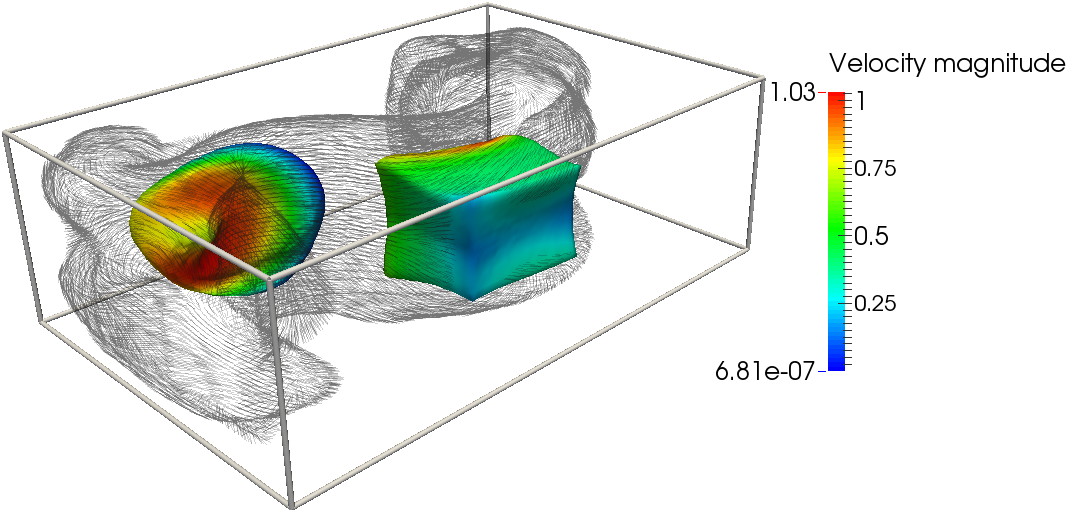
Warped surfaces
This scenario demonstrates the use of warped surfaces, a variation on the previous scenarion. Two surfaces are embedded in a 3D flow field - a box and a sphere. Next, the surfaces are warped in the direction of their normal, with a distance proportional to the flow magnitude. The resulting structures are color-coded on the flow magnitude to additionally emphasize this quantity. Finally, an isosurface of the flow magnitude is extracted, and vector glyphs are shown for seed points located on it.