Chapter 8: Domain-Modeling Techniques
Scenarios
Below are several scenarios that illustrate techniques for the processing of 2D and 3D datasets, as described in Chapter 8. As always, make sure to study also the complementary techniques described in the source code samples for Chapter 8.
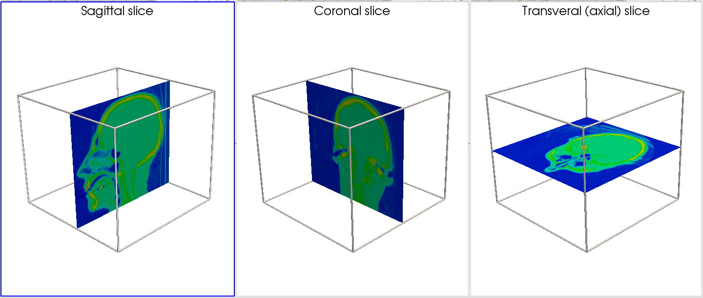
Slicing (3D volume)
This scenario demonstrates slicing 3D volumes. From a scalar volume, three axis-aligned slices are constructed (sagittal, coronal, and axial or transversal). Next, classical color mapping is used to show scalar values on these slices.
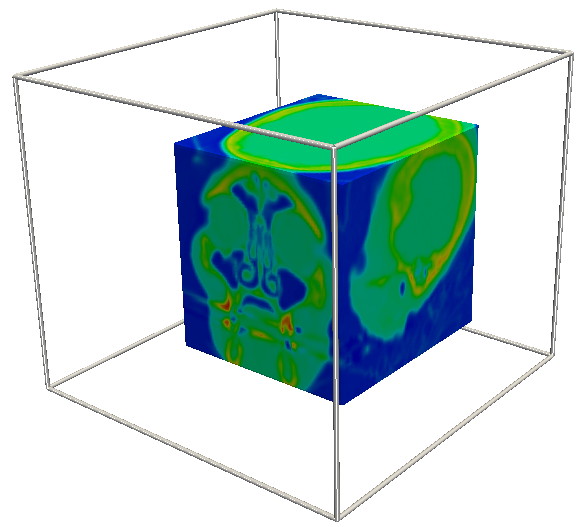
Clipping (3D volume)
This scenario demonstrates clipping 3D volumes. From a scalar volume, an axis-aligned region is selected as clip region, and extracted from the volume. Next, this region is visualized using classical color mapping.
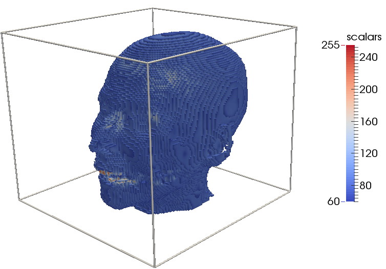
Selection (3D volume)
This scenario demonstrates selecting regions from 3D volumes based on data values. From a scalar volume, all cells are selected whose scalar values are over a given threshold. Next, the selection is visualized using classical color mapping. This effectively demonstrates the difference between threshold sets (produced by selection) and level sets (produced by isosurfaces, see the related scenarios in Chapter 5).
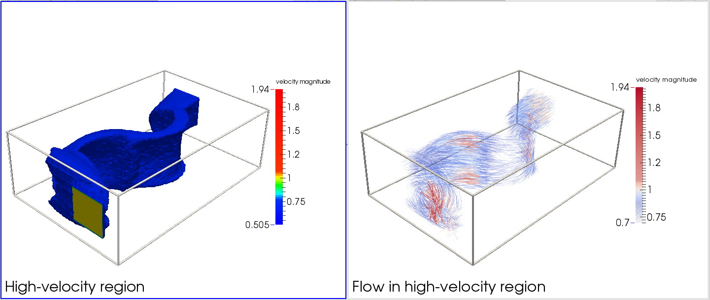
Selection 2 (3D flow volume)
This scenario demonstrates two additional variations for selecting data. Given a 3D flow volume, the first variation selects all cells where the flow magnitude exceeds a certain value. The selection is next visualized with color mapping. The second variation performs the same selection, but visualizes the selected data cells using hedgehogs. Both selections show different views of the same high-speed flow region.
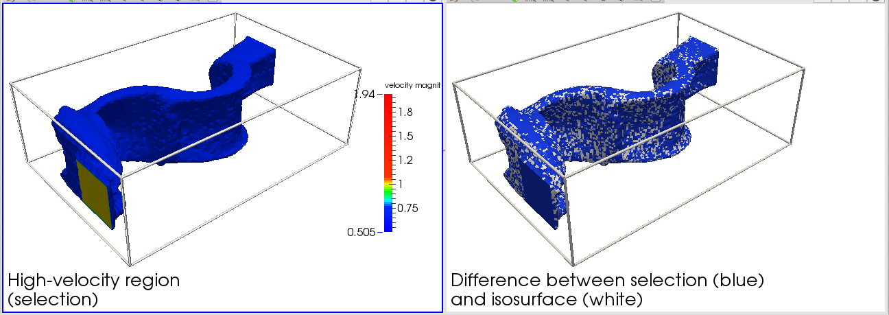
Selection vs isosurface (3D flow volume)
This scenario demonstrates the difference between selecting data (or computing a threshold set) and contouring data (or computing a level set). For the same scalar value, both structures are computed, and visualized with two different colors. The difference between the two structures becomes thus visible. Try also toggling on and off one of the structures to better highlight the difference.
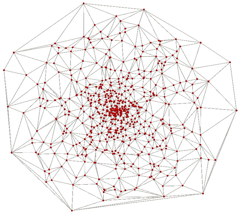
Delaunay triangulation
This scenario demonstrates the application of Delaunay triangulation to a 2D point cloud. Points in the cloud are randomly generated. The resulting Delaunay triangulation shows how the convex hull of the point cloud is covered by triangles.
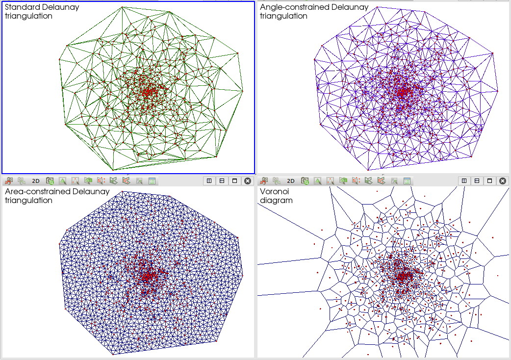
Delaunay triangulation variations
This scenario refines the previous one by showing four variations of Delaunay related operations applied to a 2D point cloud:
- the standard Delaunay triangulation
- angle-constrained Delaunay triangulation
- area-constrained Delaunay triangulation
- the corresponding Voronoi diagram
For more insight on these variations, study the Delaunay/Voronoi code samples provided for Chapter 3.
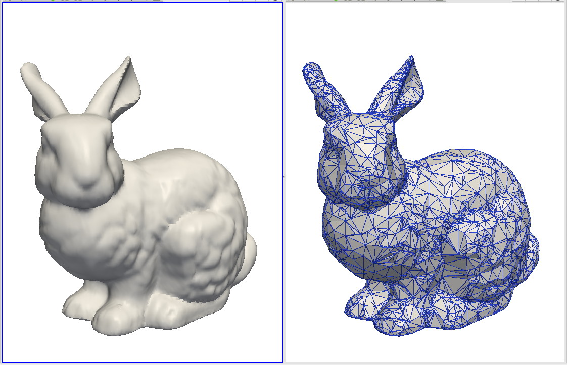
Decimation
This scenario demonstrates the use of decimation to simplify a 3D mesh. First, a simple surface mesh is loaded. Next, we visualize both the original mesh and the decimated one.
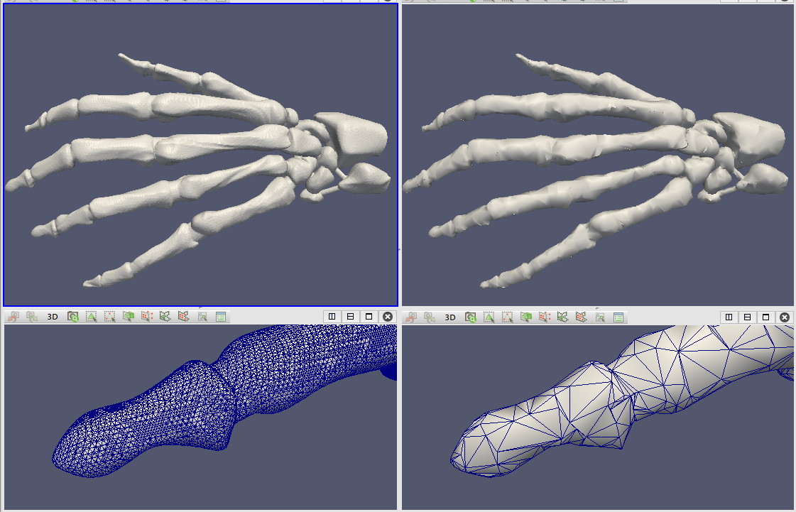
Decimation 2
This is a variation of the previous scenario, for a more complex dataset. A high-resolution mesh is loaded and next decimated. While detail zoom-ins show clear differences between the original and decimated mesh, the overview images are quite similar.
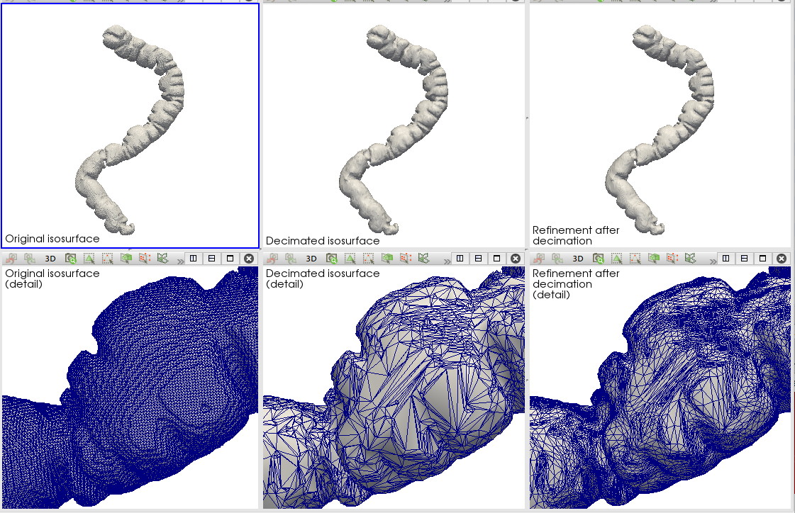
Decimation and refinement
This scenario show the combined effects of decimation and refinement. A high-resolution mesh representing the surface of a colon is loaded and visualized. Next, the mesh is decimated to yield a much smaller mesh. Finally, this smaller mesh is refined by using a mesh subdivision algorithm. The detail images show how the local mesh structure is changed by the decimation and refinement operations.
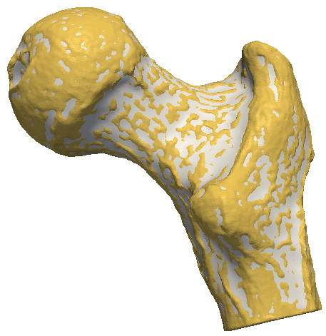
Smoothing
This scenario demonstrates the use of Laplacian smoothing to remove small-scale noise details from a 3D mesh. The original mesh (yellow) is visualized superimposed with the smoothed mesh (white). By toggling on and off the smoothed mesh in the visualization, we can see how Laplacian smoothing shrinks convex details, but inflates concave ones.
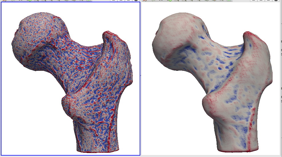
Smoothing and curvature
This scenario refines the previous one by showing the effect of Laplacian smoothing on the curvature of a mesh. The scenario visualizes side-by-side the mean curvature of the original (noisy) mesh and the smoothed mesh, using color coding. This shows how smoothing removes high-curvature regions.