Chapter 9: Image Visualization
Scenarios
Below are several scenarios that illustrate techniques for the visualization of 2D and 3D images, as described in Chapter 9. Make sure to study also the complementary techniques described in the source code samples for Chapter 9.
Distance transforms and skeletons (2D shape)
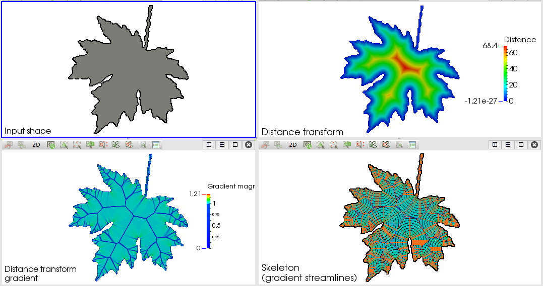
This scenario illustrates the connection between distance transforms and skeletons for a 2D shape. For such a shape, we visualize
- the shape itself
- the shape's distance transform, color-coded
- the gradient magnitude of the distance transform. Low values thereof correspond to the skeleton locations
- the isolines of the distance transform and the streamlines of its gradient. The two structures are visibly orthogonal to each other
The 2D distance transforms and skeletons used in this scenario are computed with the sample code provided for Chapter 9.
Multiscale skeletonization (2D shape)
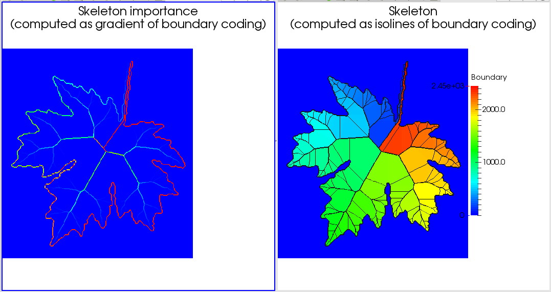
This scenario illustrates the computation of multiscale 2D skeletons. Given a 2D shape represented as a binary image, we first compute its multiscale skeleton using the AFMM method provided in Chapter 9. Next, we visualize its skeleton as the gradient magnitude of the AFMM boundary coding (for details, study the respective code). Finally, we visualize a more accurate version of the skeleton by extracting an isoline of the boundary coding scalar field.
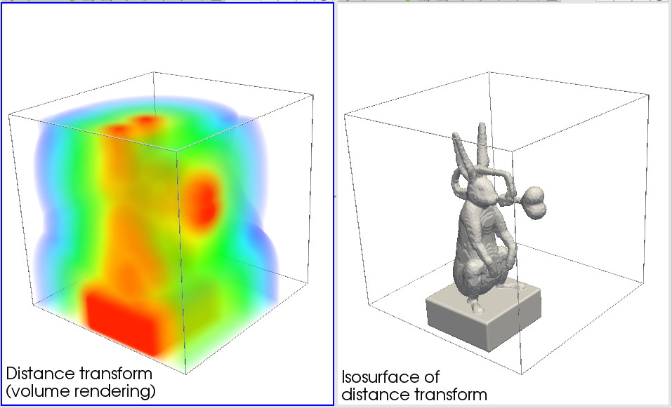
Distance transforms (3D shape)
This scenario visualizes a 3D volume encoding the distance transform of a 3D shape. The actual distance transform is computed using the sample code provided in Chapter 9. Next, we visualize this 3D scalar field using both volume rendering and isosurfacing. By changing the isosurface value, one obtains 'offsets' of the initial shape, much like when performing dilation or erosion.
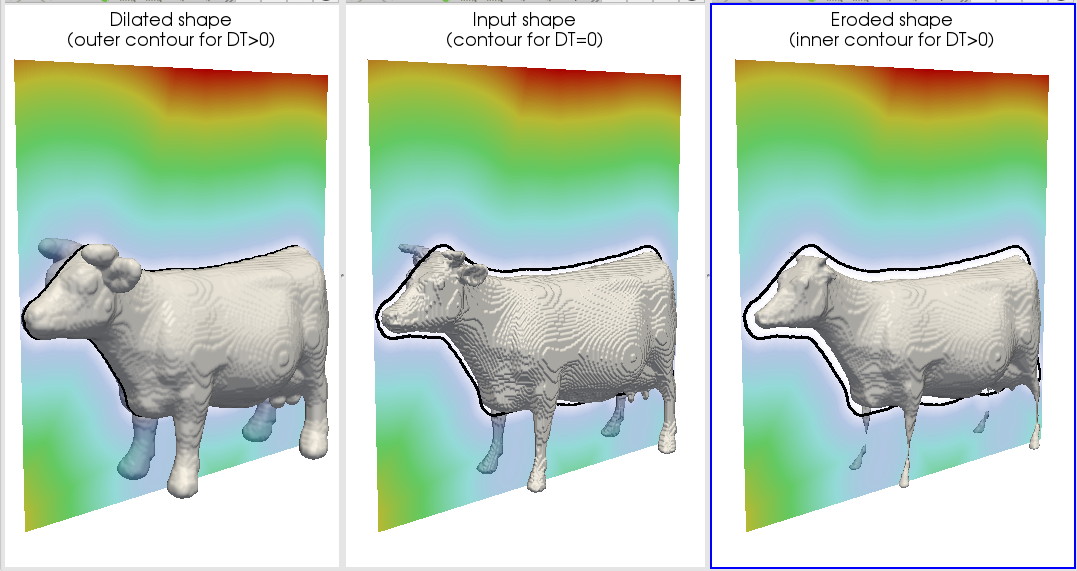
Dilation and erosion (3D shape)
This scenario illustrates how one can compute dilations and erosions of a 3D shape using its distance transform. First, we compute a 3D scalar volume encoding the shape's distance transform, using the sample code provided in Chapter 9. Next, we contour this scalar volume at various values. The effect is visualized by showing a slice plane of the distance transform with an isoline corresponding to the input shape, and the isosurfaces corresponding to several selected contour values.