Chapter 3: Data Representation
Scenarios
These scenarios illustrate the various types of grids and attributes described in Chapter 3.
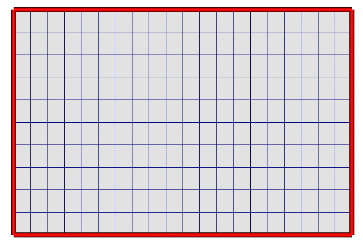
Uniform grids (2D rectangle)
This scenario demonstrates the creation of a 2D uniform grid that covers a rectangular domain.
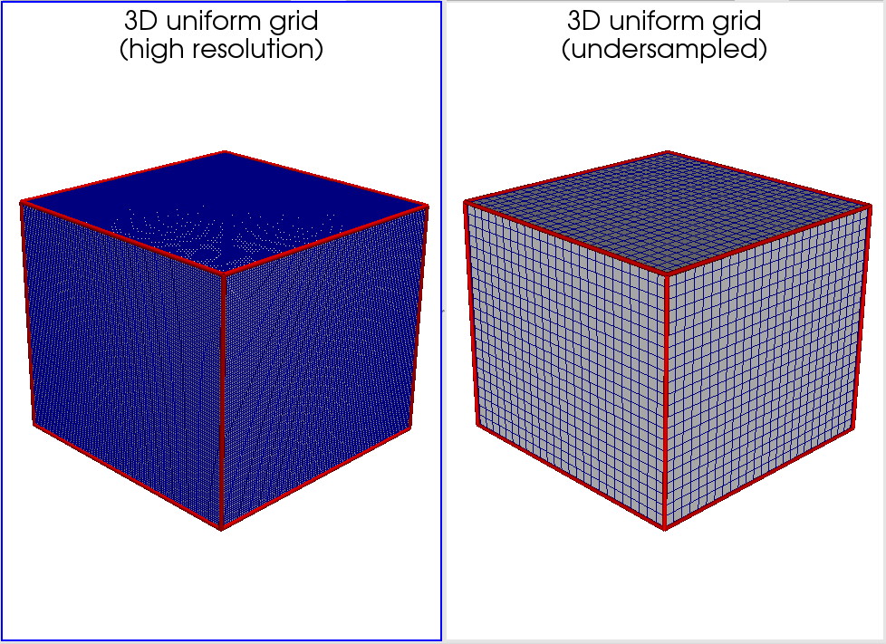
Uniform grids (3D volume)
This scenario demonstrates the visualization of a 3D uniform grid, loaded from a VTK dataset. It also demonstrates how to undersample such a dataset.
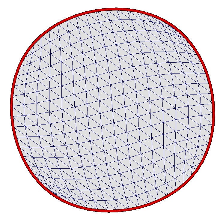
Structured grids (circle)
This scenario demonstrates the creation of a 2D structured grid that covers the interior of a circle.
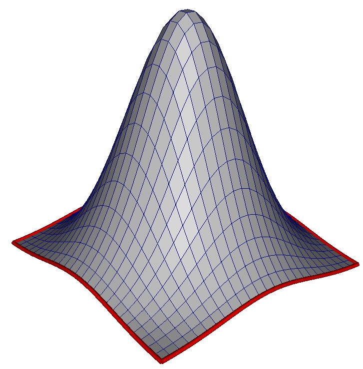
Structured grids (Gaussian)
This scenario demonstrates the creation of a 3D structured grid that represents the surface created by plotting a 2D Gaussian function.
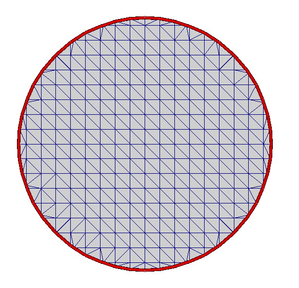
Unstructured grids (circle)
This scenario demonstrates the visualization of a 2D unstructured grid, created by Delaunay triangulation of a 2D circular area.
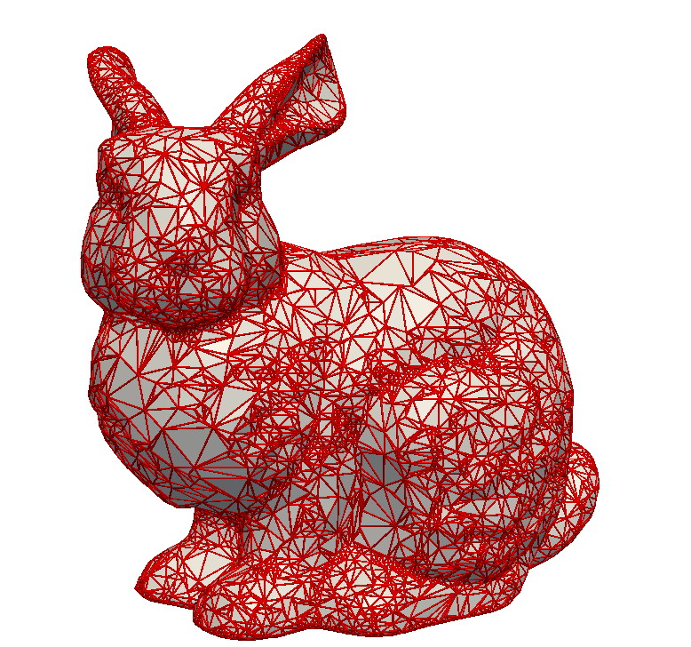
Unstructured grids (3D mesh)
This scenario demonstrates the visualization of a 3D unstructured grid, loaded from a PLY file.
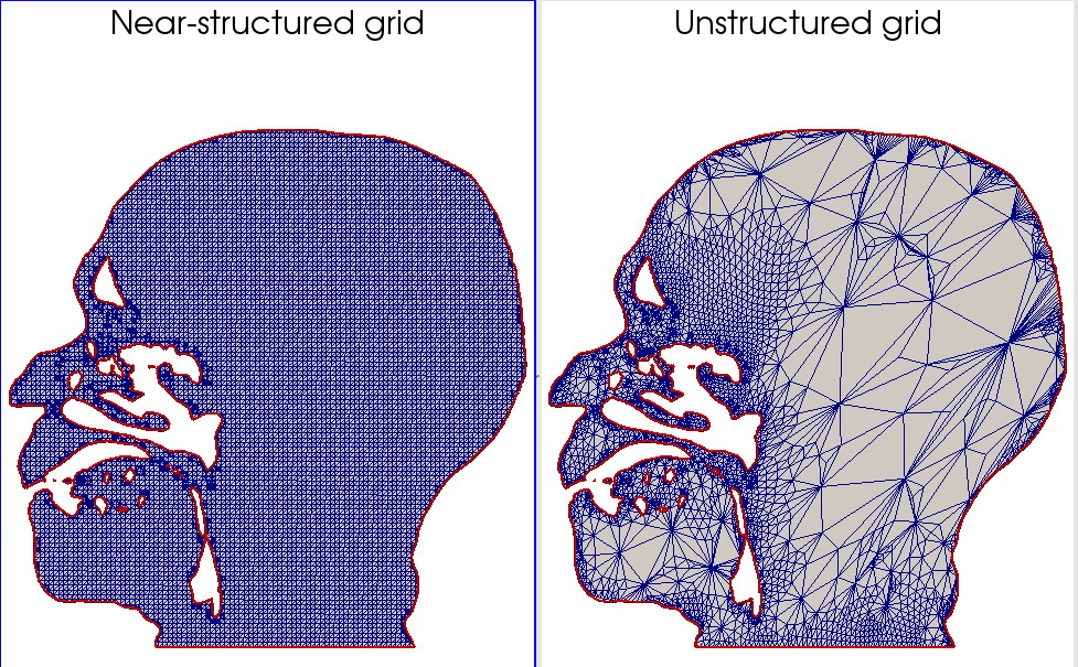
Unstructured grids (2D slice)
This scenario demonstrates the visualization of a 2D unstructured grid, created from a slice of a 3D volume. Two such grids are shown: a near-structured one, and a highly unstructured one.
Point clouds
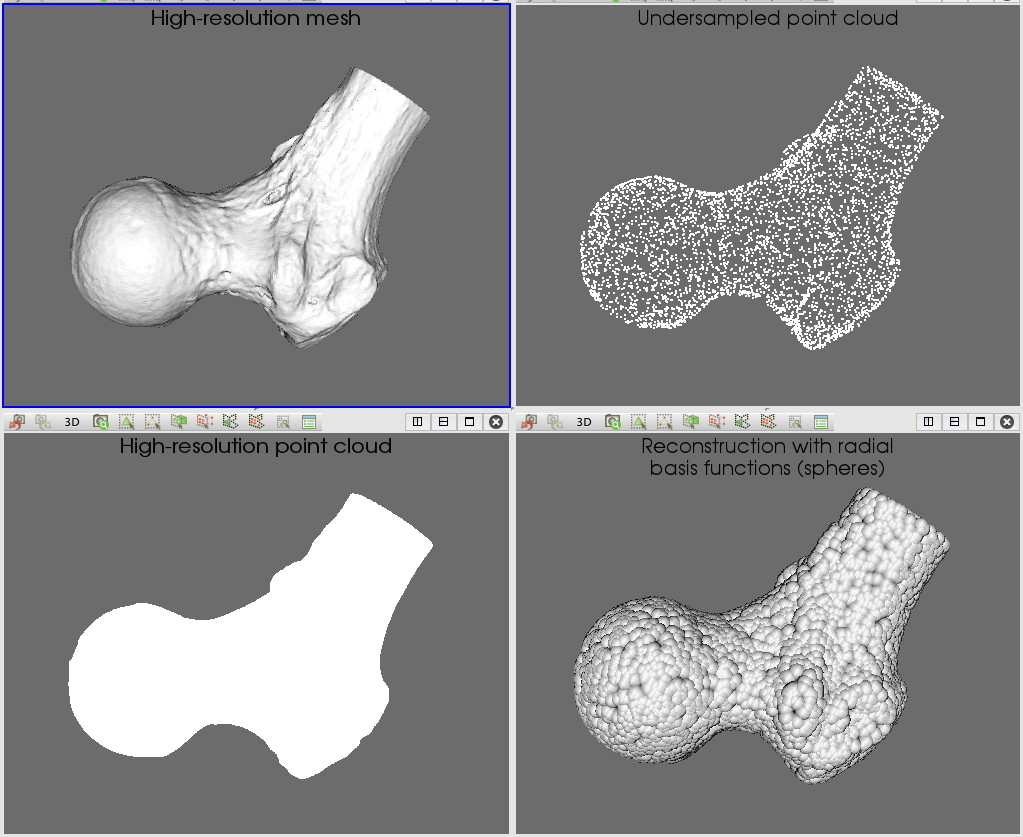
This sample demonstrates basic visualizations of unstructured 3D point clouds. The sample loads a 3D meshed surface, and next displays
- the surface, rendered with shaded polygons
- the vertices of the mesh, without shading (i.e. a point cloud)
- an undersampled version of the point cloud
- a basic reconstruction of the surface, using spheres (radial basis functions)
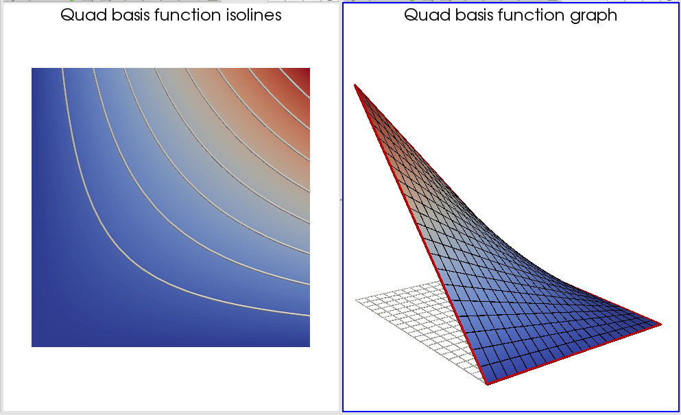
Bilinear basis functions
This sample visualizes a bilinear basis function over a 2D quad cell. The function is visualizes using color mapping, isolines, and height plots. The sample can be useful as teaching material to illustrate how such a basis function looks like.
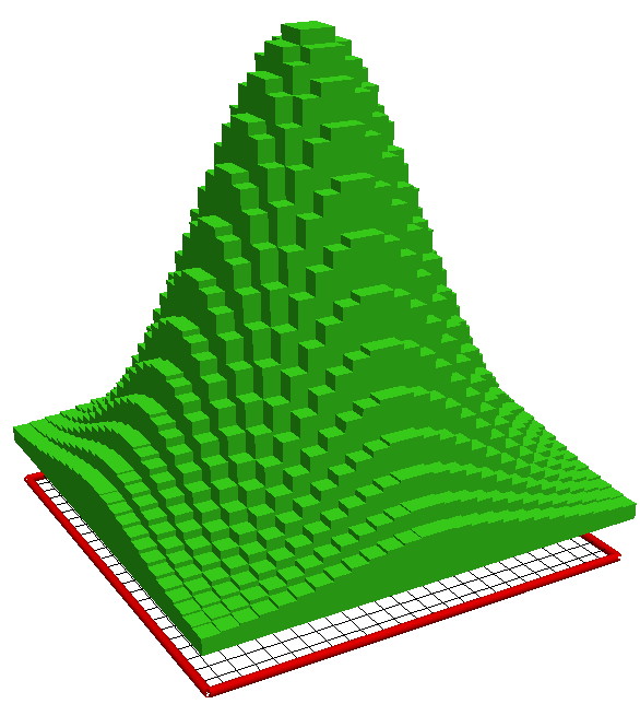
Function plot (constant basis functions)
This sample visualizes a 2D Gaussian function using constant (nearest neighbor) basis functions for the surface. The sample can be useful as teaching material to illustrate how constant basis functions look like.
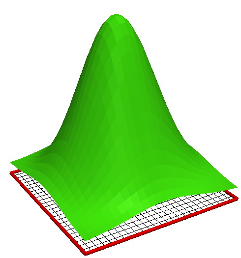
Function plot (flat shading)
This sample visualizes 2D Gaussian function using constant (nearest neighbor) basis functions for the shading (illumination). This is also called flat shading, as discussed in Chapter 2. The sample can be useful as teaching material to illustrate how what constant basis functions mean for shading.
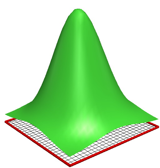
Function plot (smooth shading)
This sample visualizes 2D Gaussian function using bilinear basis functions for the shading (illumination). This is also called Gouraud shading, as discussed in Chapter 2. The sample can be useful as teaching material to illustrate how what bilinear basis functions mean for shading.
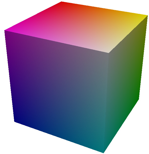
RGB color cube
This sample visualizes the RGB color cube. It can be easily changed to add annotations (e.g., labels for its vertices, or slice planes to see inside it). It can serve as teaching material to demonstrate the concept of the RGB color space.
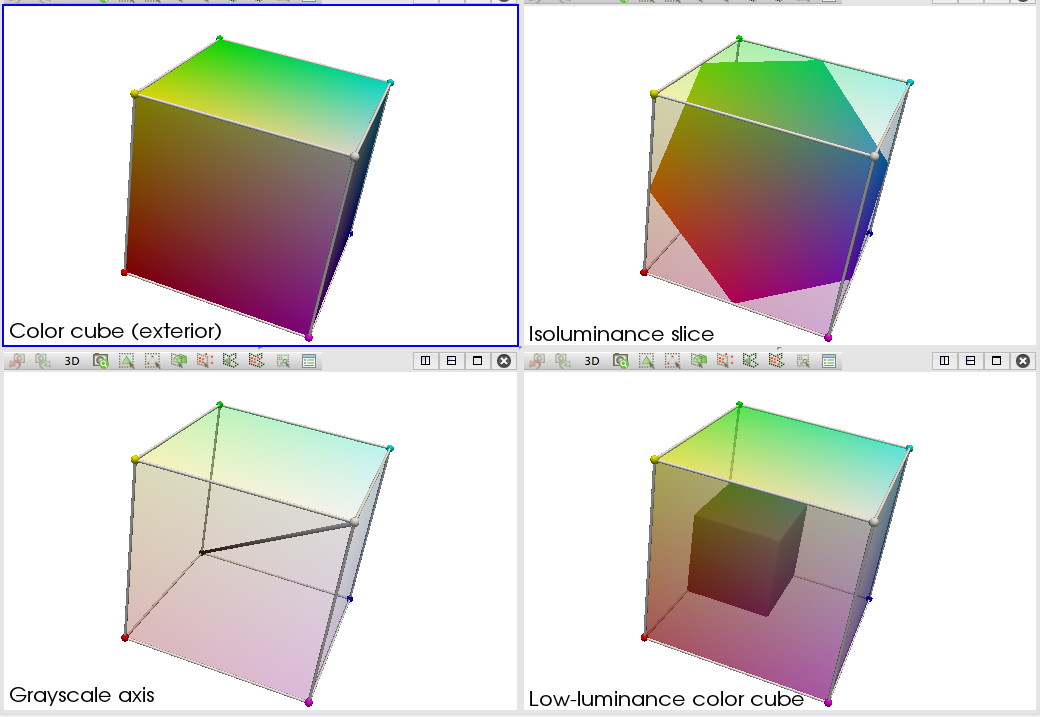
RGB color cube (enhanced)
This sample extends the previous one by adding some more exploratory visualizations of the RGB color space. The sample visualizes
- the outer surface of the RGB color space
- an isoluminance slice through the space
- the grayscale color axis
- a surface capturing low-luminance colors
The sample can serve as teaching material to demonstrate the concept of the RGB color space.