Chapter 7: Tensor Visualization
Sample programs
Curvature tensor visualization
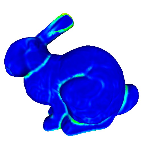
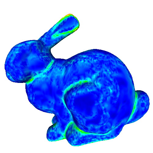
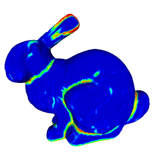
This sample demonstrates the computation and visualization of curvature tensors on 3D surfaces. Given a mesh surface, the sample estimates the eigenvectors and eigenvalues of the curvature tensor at each point p, using principal component analysis (PCA) of the covariance matrix of the point positions in a neighborhood of p. The sample also demonstrates how to find the neighbors of a point within a given radius. Eigenvalues are next visualized by color-coding. Eigenvectors are visualized by vector glyphs.
Try the sample on the provided PLY meshes! Notice how
- the major eigenvector is nicely aligned with the salient edges on the surface;
- the medium eigenvector is orthogonal to such edges;
- the minor eigenvector is aligned the surface normal.
Next, vary the size of the neighborhood, and notice how surface details at various scales are filtered out.
Surface classification
This sample demonstrates the computation and visualization of surface classifier metrics. Such metrics characterize points of a 3D surface in terms of their being part of flat areas or highly curved areas (such as edges or corners). Classifiers are estimated based on the PCA analysis of the surface curvature tensor estimated in the previous sample. The following classifiers are demonstrated:
- surface variation (Pauly, 2003)
- planar anisotropy (Westin, 1997)
- momentum-based classifier ((Clarenz, 2004)
Try the sample on the provided PLY meshes! Notice how
- the different classifiers achieve different performances in detecting flat or highly-curved surface areas
- all classifiers depend on the neighborhood size
This sample also demonstrates how to select surface neighborhoods on a 3D surface, defined by a given centerpoint and radius, in a more robust way than using the 3D point-searching shown in the previous sample.
3D tensor field representation
This sample demonstrates how to implement a 3D tensor dataset. The sample is based on the Volume dataset representation described in Chapter 10. It provides the basic infrastructure required for
- representing 3D tensor fields (having an additional confidence value)
- reading 3D tensor fields from the popular open-source NRRD format
- extracting a tensor component and saving it as a 3D scalar field
Tensor representation (part 1)
Tensor representation (part 2)
Tensor representation (part 3)
Tensor representation (part 4)
Tensor representation (part 5)
Note: Since the sample is quite large, we provide it as a 5-piece multipart ZIP archive. To unzip this, rename the first four parts to filename.z01..filename.z04 and the fifth part to filename.zip. After that, you can use any unzip utilities on filename.zip.
This sample can be easily combined with the isosurface code (Chapter 5) and the voxel-surface rendering code (Chapter 10), to render specific tensor components.
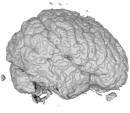
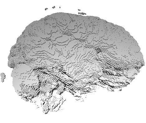
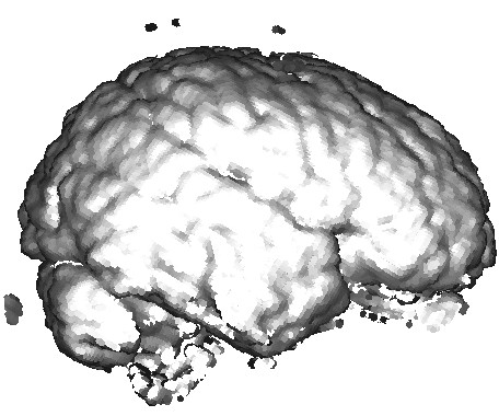
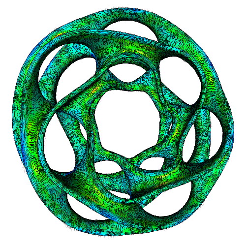
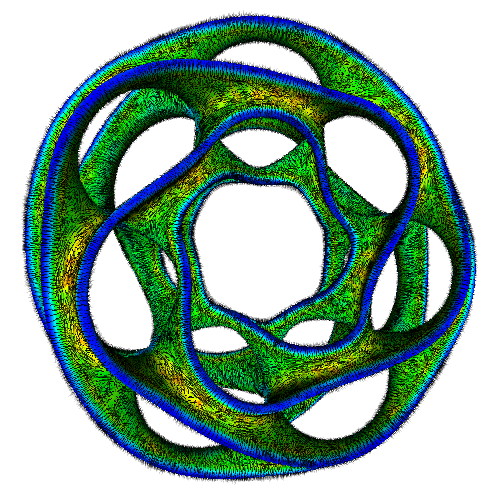
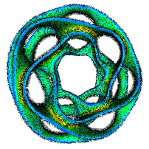
The three images above illustrate this. All images extract the confidence component of a 3D DT-MRI (diffusion-weighted MRI) tensor field, using the command
sampleTensorComponents DATA/gk2-rcc-mask.nhdr -o confidence confidence.fld
Next, we visualize this field as follows:
- left image:
sampleIsosurface confidence.fld(see Chapter 5) - middle and right images:
sampleVoxelSurface confidence.fld(see Chapter 10)
Note: DTI tensor data: courtesy of G. Kindlmann.
Tensor metrics
This sample demonstrates the processing and visualization of 3D DTI (diffusion-weighted MRI) tensor fields by a number of techniques:
- computing the eigenvalues and eigenvectors of the field
- computing the mean diffusivity and fractional anisotropy
- extracting axis-aligned 2D slices from the 3D field
- visualizing slices with scalar color-coding and vector directional color-coding (similar to Figures 7.5 and 7.7)
- masking the visualized data by a confidence field
- constructing 2D uniform grids with cell-based scalar and vector data attributes (as opposed to the vertex-based attributes demonstrated in Chapter 3.
- saving tensor metrics to third-party file formats (AVS and VTK)
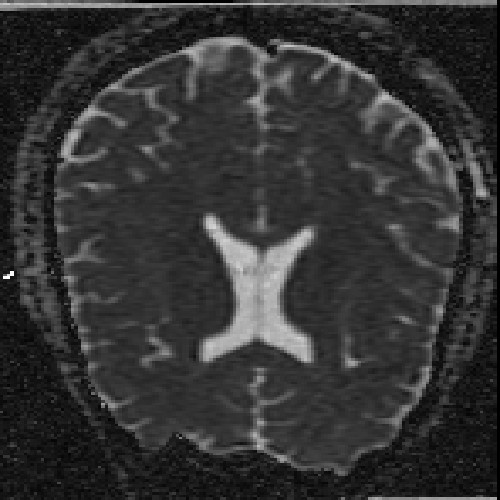
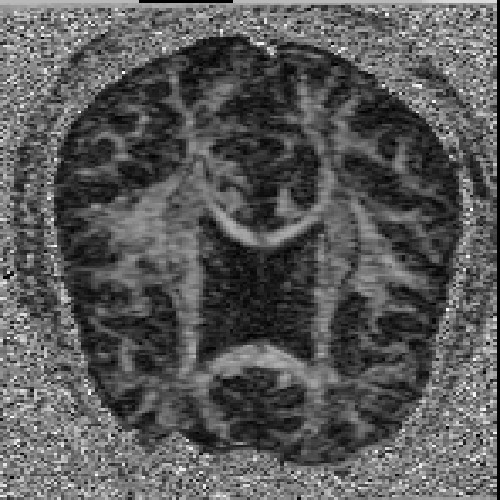
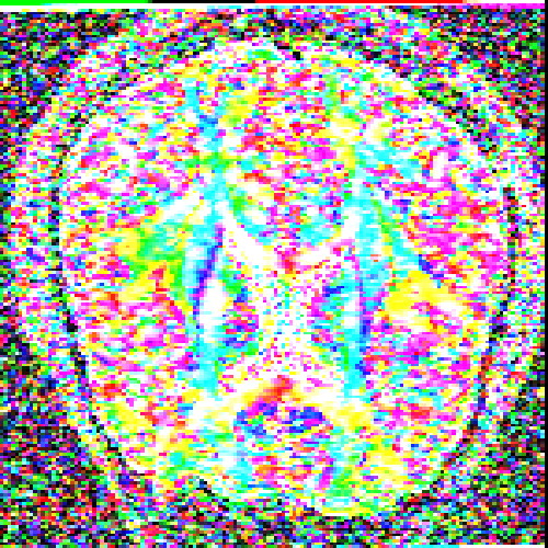
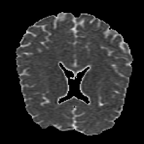
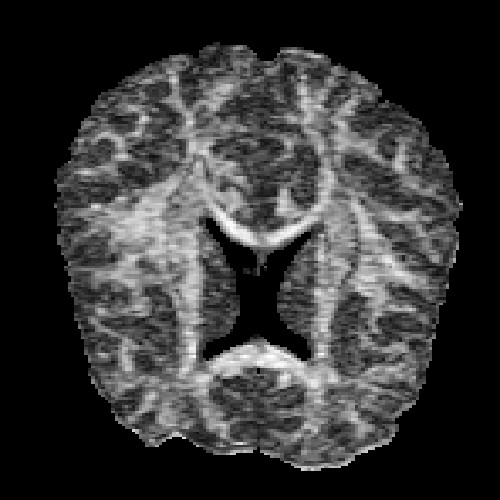
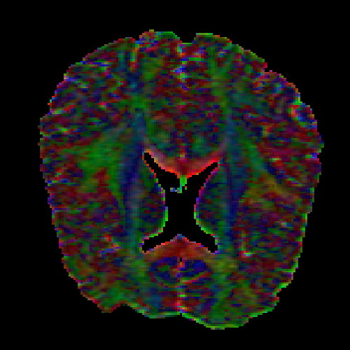
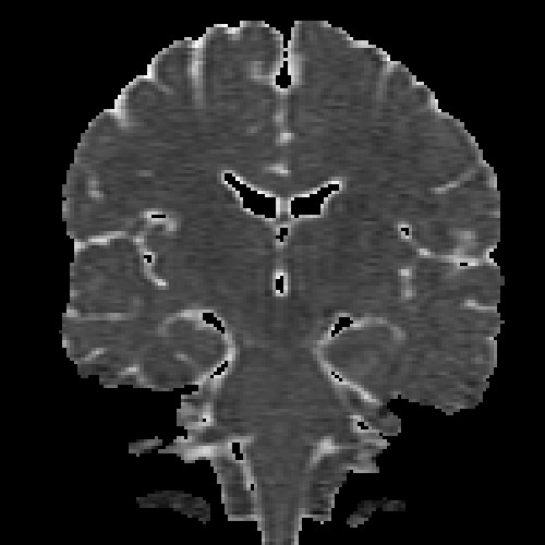
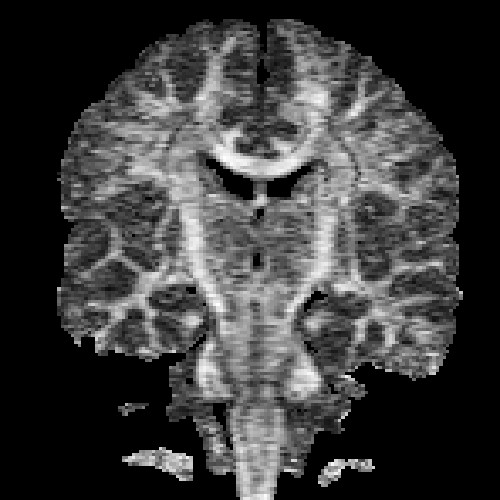
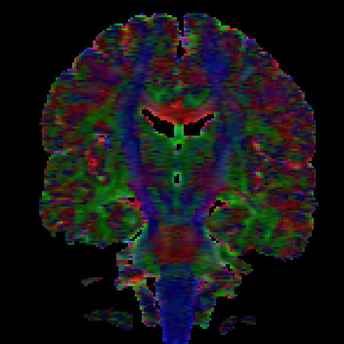
The images above (columns, from left to right) show the mean diffusivity, linear anisotropy, and color-coded direction of the major eigenvector of the DTI dataset provided in the previous code sample. The three image rows show:
- top row: The raw computation of the above metrics. As visible, noise artifacts appear in areas where the DTI measurements are uncertain, such as outside the head.
- middle row: The above metrics, masked by the measurement confidence. This significantly reduces noise.
- bottom row: Identical to the middle row, but slices are taken from a different direction.
Note: The DTI dataset for this sample is not provided in the ZIP file, since it is the same as the one for the previous sample. As such, download it separately either by downloading the previous sample or directly from the source, and place it in the DATA directory of this sample.
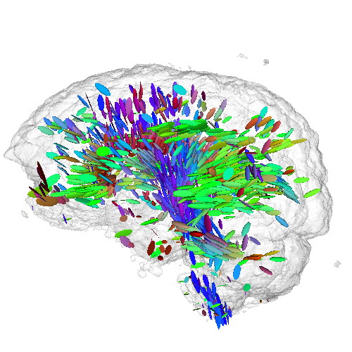
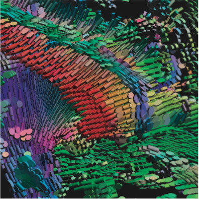
Tensor glyphs
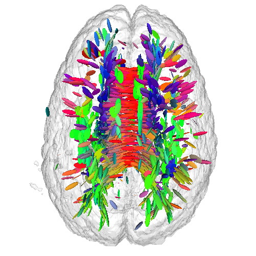
This sample demonstrates the visualization of a 3D DTI field using tensor glyphs. The sample
- uses the previous tensor metrics sample code to compute the eigenanalysis of a tensor field
- computes a set of dense seed points in locations of high anisotropy and confidence of the tensor field
- for each seed point, creates a 3D ellipsoid whose half-axes are oriented along the tensor's eigenvectors and
scaled with the tensor's respective eigenvalues
- draws the tensor glyphs at the sample points, color-coded by the major eigenvector direction
Additionally, a half-transparent isosurface of the tensor confidence field is displayed around the tensor glyphs to offer additional orientation cues.
Note: The DTI dataset for this sample is not provided in the ZIP file, since it is the same as the one for the previous sample. As such, download it separately either by downloading the previous sample or directly from the source, and place it in the DATA directory of this sample.
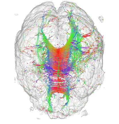
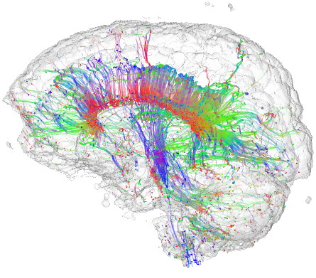
Tensor streamlines
This sample demonstrates the visualization of a 3D DTI field using streamlines of its major eigenvector field. The sample
- uses the previous tensor metrics sample code to compute the eigenanalysis of a tensor field
- extends the streamlines sample from Chapter6 to trace streamlines in a 3D vector field represented as a Volume. This also demonstrates how to perform cell-to-vertex data conversion on a 3D uniform grid, and how to perform trilinear interpolation on such a grid
- color-codes streamlines using the directional-coding presented in the tensor metrics sample above
Streamlines are seeded in regions of high confidence and anisotropy, to maximize their relevance. Additionally, a half-transparent isosurface of the tensor confidence field is displayed around the streamlines to offer additional orientation cues.
Note: The DTI dataset for this sample is not provided in the ZIP file, since it is the same as the one for the previous sample. As such, download it separately either by downloading the previous sample or directly from the source, and place it in the DATA directory of this sample.
Tensor processing toolkit
For those interested in experimenting with a wider range of more complex methods for tensor field processing and visualization, Teem is a good solution. Teem is an open-source framework (libraries and command-line tools) that offers methods for the
- generation of simple sample 2D and 3D tensor fields
- basic processing of nD raster data (e.g. clipping, resampling, interpolation, filtering)
- tensor visualization with glyphs and volume rendering
Teem can form the basis of a multitude of small-to-medium size student projects spanning tensor visualization, image processing, and volume visualization. Using Teem requires being handy with Unix/Linux command-line tools, shell scripts. Understanding Teem requires a fair knowledge of programming in C.
Teem is freely downloadable (external link).