Chapter 7: Tensor Visualization
Scenarios
Below are several scenarios that illustrate techniques for the visualization of 3D tensor datasets described in Chapter 7. As always, make sure to study also the complementary techniques described in the source code samples for Chapter 7.
Extremal curvature directions
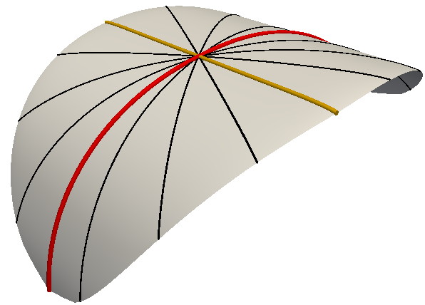
This scenario illustrates the curvature tensor for a 3D surface. For such a simple surface, we construct a number of slice planes that 'rotate' along its normal at a given point. For each such slice plane, we visualize its intersection with the surface, which yields a planar curve. The two planes containing the curves having the maximal, respectively minimal, curvatures at the considered point correspond to the directions of the major, respectively minor, eigenvectors of the curvature tensor.
Tensor streamlines
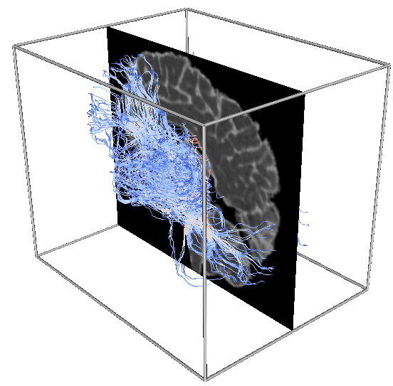
This scenario illustrates the visualization of 3D DTI (diffusion-weighted MRI) tensor fields using streamlines. Given a DTI volume, we first compute two derived fields from it
- the mean diffusivity (a 3D scalar field)
- the major eigenvector (a 3D vector field)
Next, we mask both fields with the confidence of the tensor field measurements. This eliminates from further visualization all locations where the tensor data is unreliable.
Finally, we visualize the major eigenvector field using 3D streamlines. For orientation cues, we add a 2D slice showing the mean diffusivity field.
Note 1: The computation of the derived tensor quantities is done using the tensor metrics code sample presented in Chapter 7.
Note 2: Original DTI tensor data: courtesy of G. Kindlmann.